Demo: The pole balancer on DANNA

James S. Plank.
Summer 2016

This is a classic application from control theory. A pole is to be balanced on a cart that can move horizontally within a fixed area. The pole has a mass on its top. The pole starts in some imbalanced starting state, at some angle from vertical, rising or falling at some velocity. The goal of the system is to apply periodic forces to move the cart left or right, to keep the pole from falling, and to keep the cart from moving beyond its boundaries.

Our goal is for our neuromorphic models to "solve" instances of the pole balancing problem. Before we get to that, though, it's good to visualize the problem. In the video below, we start with a stationary cart, with the pole just a little to the right of vertical. (The angle from the pole to vertical is 0.001 radians). If you push the play button, you'll see that the pole starts falling to the right, slowly at first, and then faster, until it reaches an angle that we deem too big (0.209 radians). When that happens, we turn the pole red, and show the failing angle:

Our simulation is set up so that every 1/50s, one can apply a force to the cart to move it either to the left or to the right. The force is always the same. The goal is that whoever is applying the force can keep the pole balanced and can keep the cart between the borders of its track.

The following video shows another example of the pole balancer. Here, the starting point is at a greater angle from vertical (0.15 radians), so to keep it from falling too much, we apply force to the right. Unfortunately, we never apply force to the left, so even though the pole never falls too much, the car rams into the right wall!

Now, to have a neuromorphic implementation solve the pole balancing problem, we need to translate instances of the problem into charge events that are input to the neuromorphic implementation. Then, we need to interpret the output charge events from the neuromorphic implementation, and turn them into input for the pole balancing problem.

Our solution works as follows. Let's use the DANNA neuromorphic model as an example. Every 1/50s, we communicate the state of the pole balancing to the DANNA system, which has been programmed by evolutionary optimization to solve the problem. This state is composed of four parameters:

The x position of the cart.
The x velocity of the cart.
The angle θ of the pole from vertical.
The velocity of how the angle θ is changing.

Our DANNA network has 12 input neurons, three for each of these parameters. The values of each parameter are split into three bins. For example, the x position of the cart is split into "Left", "Middle" and "Right." When the state of the system is input into DANNA, a fixed charge is fired into the neurons corresponding to the four parameters.

The DANNA network then runs for 100 cycles, and there are two output synapses, whose firing events are counted. If one of them fires more than the other, then the result of the simulation is to apply force to the cart, to the left. If the other fires more, then the result of the simulation is to apply force to the cart, to the right. If the two fire equally, then no force is applied.

The picture below summarizes:

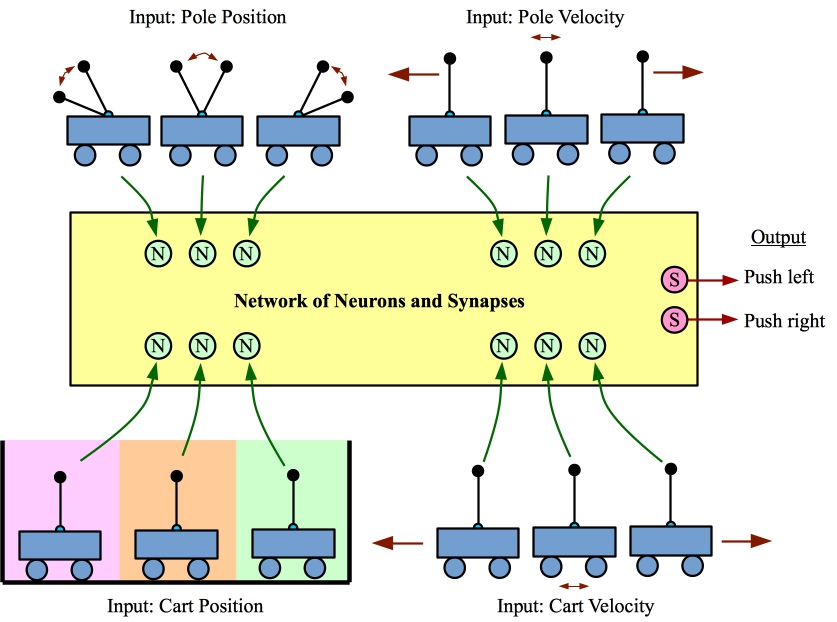Example of turning an instance of the Inverted Pendulum on a Cart into input and output that our networks can understand.

And the picture below shows a 15 X 15 DANNA network that has been programmed to solve the problem. In the picture, the neurons are light blue, and the synapses are tan. The picture shows the 12 input neurons, and the two output synapses. Yes, some of the inputs are not connected to anything -- more on that later.

Watch DANNA Balance the Pole for a Minute

The following video shows DANNA balancing the pole for a minute. This is just a clip -- on this input, the DANNA network keeps the pole balanced within the given boundaries for over a simulated week (we stopped running the simulation).

As you play the video, you'll see the positions and velocities of the cart and the pole go through various combinations of "high/middle/low." You'll also see the various states of the DANNA network that keep the pole balanced. In the video, we highlight neurons and synapses that fire in the 100-cycle intervals that translate input into output. These are highlighted by putting a dark border around the element.

The following video shows the first second of the above video, but slowed down so that each timestep takes a second, rather than a 50/th of a second. You can use this video to walk through the annotated examples that we give below.

Example 1 - Showing input and output with DANNA.

In the first screen shot, we show the starting state of the pole balancing simulation, plus how DANNA has reacted to the first 100 cycles. First, you can see how the state of the simulation is transmitted to the input neurons of DANNA. For example, the fact that the x value is in the "medium" state is communicated by pulsing input to the second neuron in the leftmost column.

You can also see how various neurons and synapses fire in the interior of the DANNA array. Most importantly, you can see that the synapse on the right side that corresponds to "pulse the cart to the right" has fired. Therefore, at the next interval, the cart will be forced to the right:

Very little has changed from the previous screen shot to this one; however, you can see that the cart has been forced to the right, which results in the cart having velocity along the x direction (0.192686 units per second, if you can read the tiny print at the bottom of the green panel), and the pole having velocity as well (-0.241804 radians per second).

As before, the "pulse cart to the right" synapse is firing, which means that the cart will continue to be pushed to the right at the next time step.

By now, the observant reader will have noticed that several of the input neurons aren't connected to anything. In particular, the input neurons for low x, middle x, low x velocity, middle theta, and middle theta velocity have no synapses coming out of them. That means that these input values are ignored, yet this DANNA network still solves the pole-balancing problem!

We are going to skip a time-step, and go to time-step 0.06 next:

There are two things to note about this screen shot. First, the theta velocity parameter has changed from the "middle" state to the "low" state. As such, its input neuron has changed. Second, although charge has gone through various neurons and synapses, neither output synapses is firing, so on the next step, there will be no pulse to the cart:

At time 0.10, theta's velocity has moved from the "low" state back to the "middle" state.

This is the same state of the system as in timesteps 0.00 through 0.04. However, you'll notice that unlike those timesteps, the output synapses here are not firing. Go double-check that -- in the screen shot above for states 0.00 and 0.02, the four parameters are in the same state, yet in those timesteps, the "pulse to the right" synapse is firing, and here, it is not.

The reason is that the neurons and synapses compose a form of memory from state to state, and their internal states at timestep 0.10 are different from what they were at, for example, timestep 0.00, which has caused the output synapses not to fire at timestep 0.10.

This is one of the features that makes our spiking neuromorphic models different from conventional neural networks in general, and Deep Learning in particular. A Deep Learning system does not have a temporal component, which means that if Deep Learning to be applied to this problem, each timestep would have to be an independently solved problem. Deep Learning, in this case, would be equivalent to a Python program with 3⁴ = 81 if statements.

At time 0.12, the input parameters remain the same, but the output synapse fires again, so the cart will be pulsed to the right at the next timestep.

Example 2 - More subtle things that you might not see if we didn't point them out.

We'll start at timestep 0.14, where x velocity moves into the high state, and theta velocity moves into the low state:

You'll note that the input neuron corresponding to x velocity is not firing. The reason is that each input pulses in 10 units of charge. The threshold for the input neuron is 57, so 10 units of charge won't make it fire. That neuron needs five more input pulses for the charge to exceed its threshold so that it fire. The x velocity parameter stays the same for the next five timesteps, so indeed, at timestep 0.24, the neuron fires:

Our next screen shot is from timestep 0.36, where the cart and pole finally get into a position when the "Pulse Left" synapse fires:

You can see the pulse at the next timestep (0.38). This timestep is interesting as well, because you can see neuron/synapse outlines of both red and black. In this picture, the red outlines denote that the neuron/synapse fired once during the 100-cycle interval, adn the black outlines denote that the neuron/synapse fired twice.

Skipping foward to timestep 0.50, here you see that both output synapses have fired in the 100 cycles.

Since the "pulse left" synapse has fired twice (black outline), but the "pulse right" synapse has fired only once (red outline), on our next timestep, we will pulse the cart to the left. Here is that timestep (0.52):

You can see that the "pulse right" synapse has fired twice, and the "pulse left" synapse has fired just once, so in the next timestep (0.54), the cart will be pulsed to the right:

And finally, during timestep 0.54, the two output synapses each fired once, so there will be no pulse to the cart on the next timestep (which I don't picture).

A few more videos from different starting positions

This first video shows a 10-second example where the cart is to the far left (x = -2.35), and its angle is theta = 0.18:

And the second shows 10-second example where the cart is to the far right (x = -1.80), its velocity is going to the right (x velocity = 0.20), and its angle velocity is falling to the right (theta velocity = 0.20):